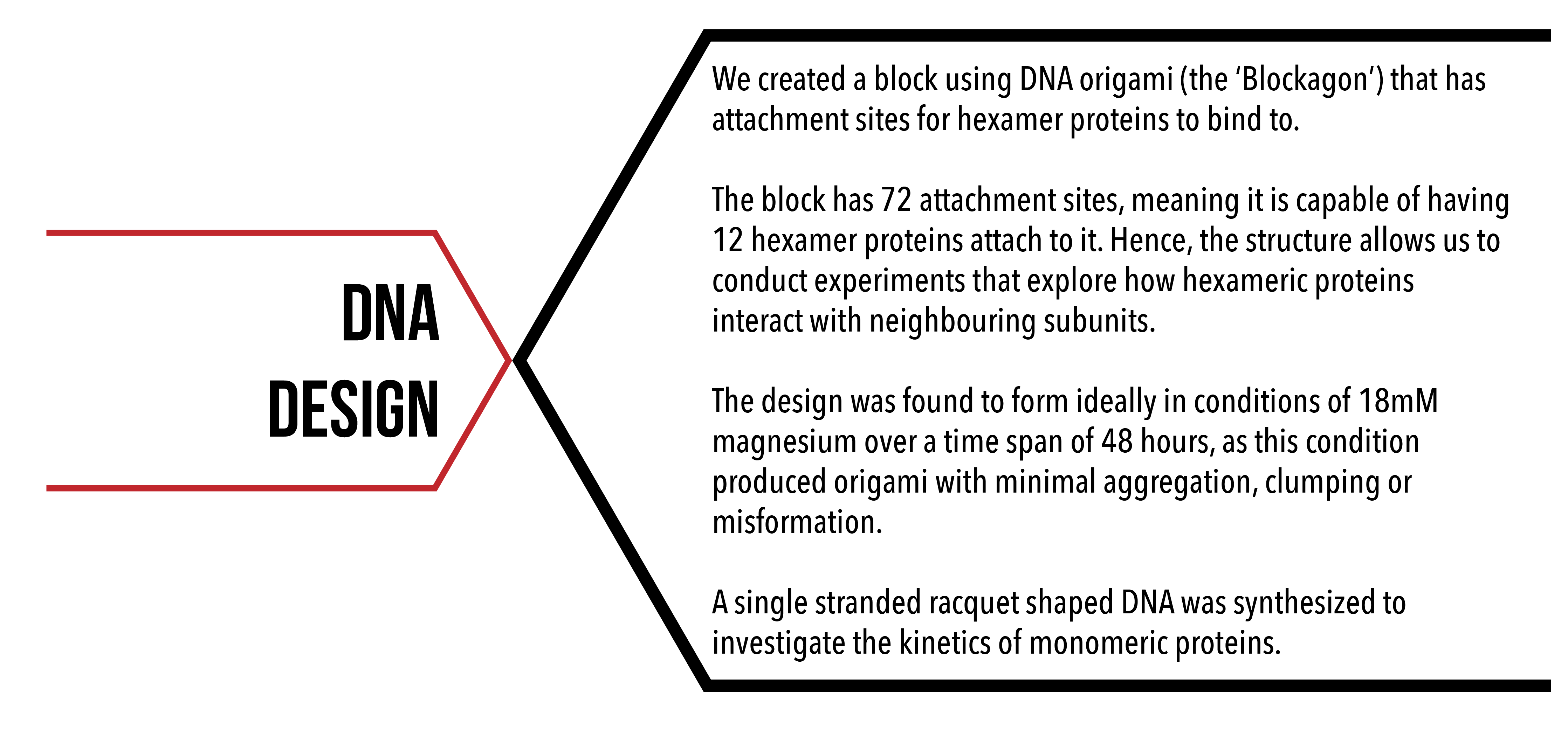
Figure 1: DNA Origami with Extensions for Binding

The technique of DNA origami was publicised by Paul Rothemund’s paper ¹, “Folding DNA to create nanoscale shapes and patterns” in 2006. Before his findings, the task of creating nanoscale sized biological devices was incredibly energy consuming as well as being a difficult to control process.

DNA origami works by folding a circular strand of DNA that serves as a backbone. Oligonucleotides, known as staple strands, then hybridise to the backbone which cause it to fold in specific sections.

Figure 2: DNA Folding Mechanism

By using a backbone to facilitate the formation of origami, the process of creating a structure becomes simple. The predictability of DNA’s pairing rules and its programmability means that structure’s staples and scaffold will self-assemble into its lowest energy state, and hence most stable state. ¹

This was first supported by Rothemund’s publications of two-dimensional shapes which he created with the DNA origami technique. These shapes included stars, triangles, and even a smiley face, demonstrating that DNA can be designed into specific structures. ¹

Since these findings in 2006, the technique of DNA origami has grown to the point where we are now able to create much more complex designs and in three-dimensional space. Concurrently, more sophisticated design and analysis tools have developed, meaning that creating specific and accurately formed DNA structures is simpler than ever. ²

We aimed to make a DNA scaffold that would allow for as many protein hexamers to bind to. For this to happen, we created a structure with a large flat surface while also ensuring that the stability of the structure was not compromised. We also aimed to create a single stranded DNA structure for protein monomers to bind to so that we could obtain kinetic data via SPR experiments

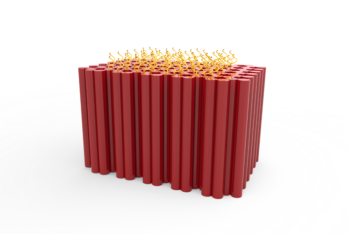
Within a full revolution of DNA there are 10.5 base pairs. Hence, 7 base pairs completes 240 degrees of rotation.

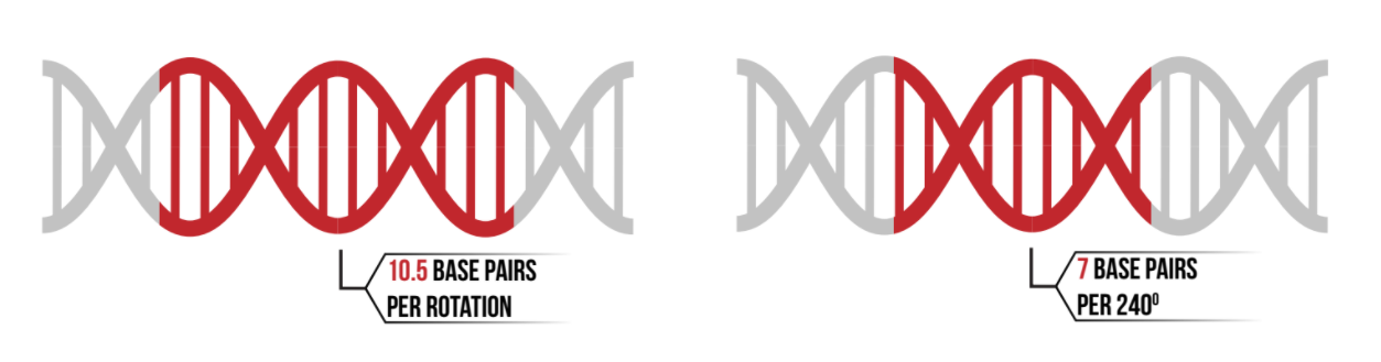
Figure 3: DNA Rotations and Base Pairs

If two parallel helices run alongside with each other, there is the chance for DNA to cross over from one helix to the other helix due to the rotation and consequent relative distance of the helices. This only occurs on certain bases of the DNA and will only occur if the structure is designed to do so i.e. the DNA will not cross over spontaneously. These crossovers are positioned such that twist strain is minimised in the structure. ³

Figure 4: DNA Cross-over

As mentioned, 7 base pairs in a helix rotates 240 degrees. This means that for 14 base pairs, and 21 base pairs, 480 and 720 degree of rotation are completed respectively. This causes a helix to have 3 distinct equally spaced angles where cross overs can occur with neighbouring helices as seen in Figure 5.

This results in a honeycomb lattice formation of helices as each helix can form crossovers with the 3 neighbouring helices as shown in Figure 6.

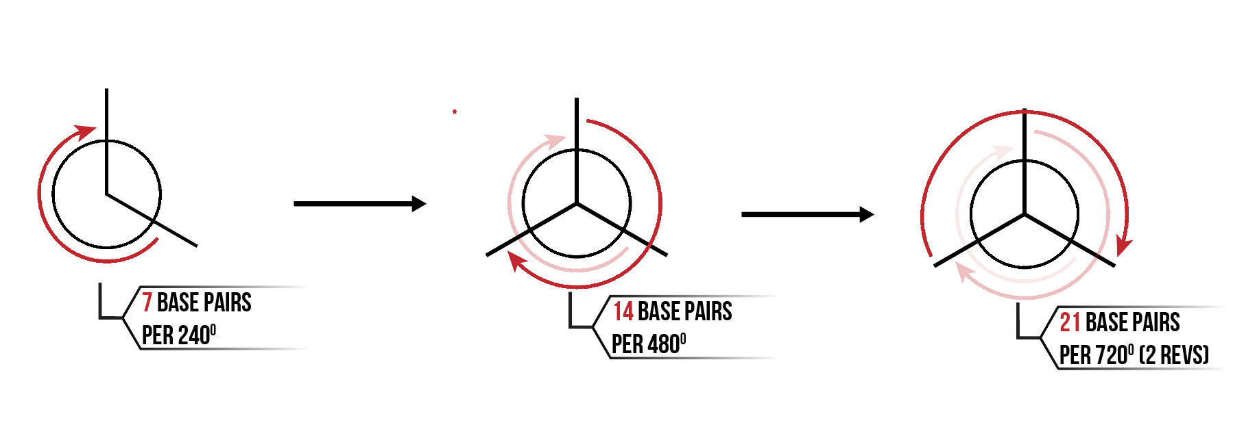
Figure 5: DNA Rotations

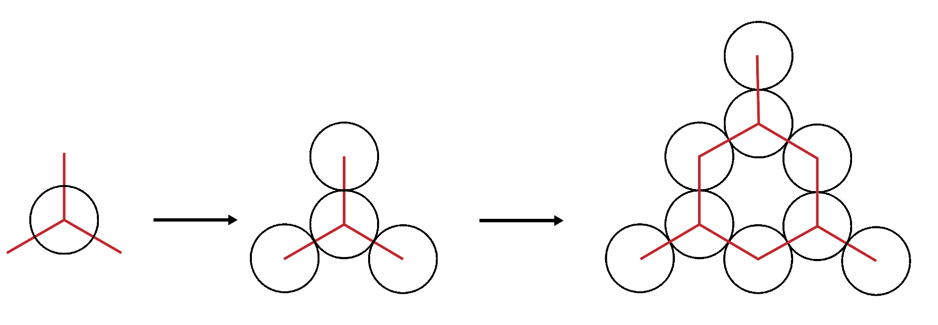
Figure 6: DNA Honeycomb Lattice

For us to create a structure capable of maximising the amount of hexamer proteins that can attach to it, we were required to create a structure with a large flat surface. While also being restricted to the length of the m13a backbone (7249 base pairs) ⁴, this meant creating a shorter structure to allow for a larger area for attachments.

However, a shorter structure meant there were less instances of DNA crossovers, hence creating a less stable structure. The challenge for us was to ensure that a suitable compromise was found between the amount of attachment sites and the stability of the structure. The final dimensions of the design are shown in Figure 7. ²

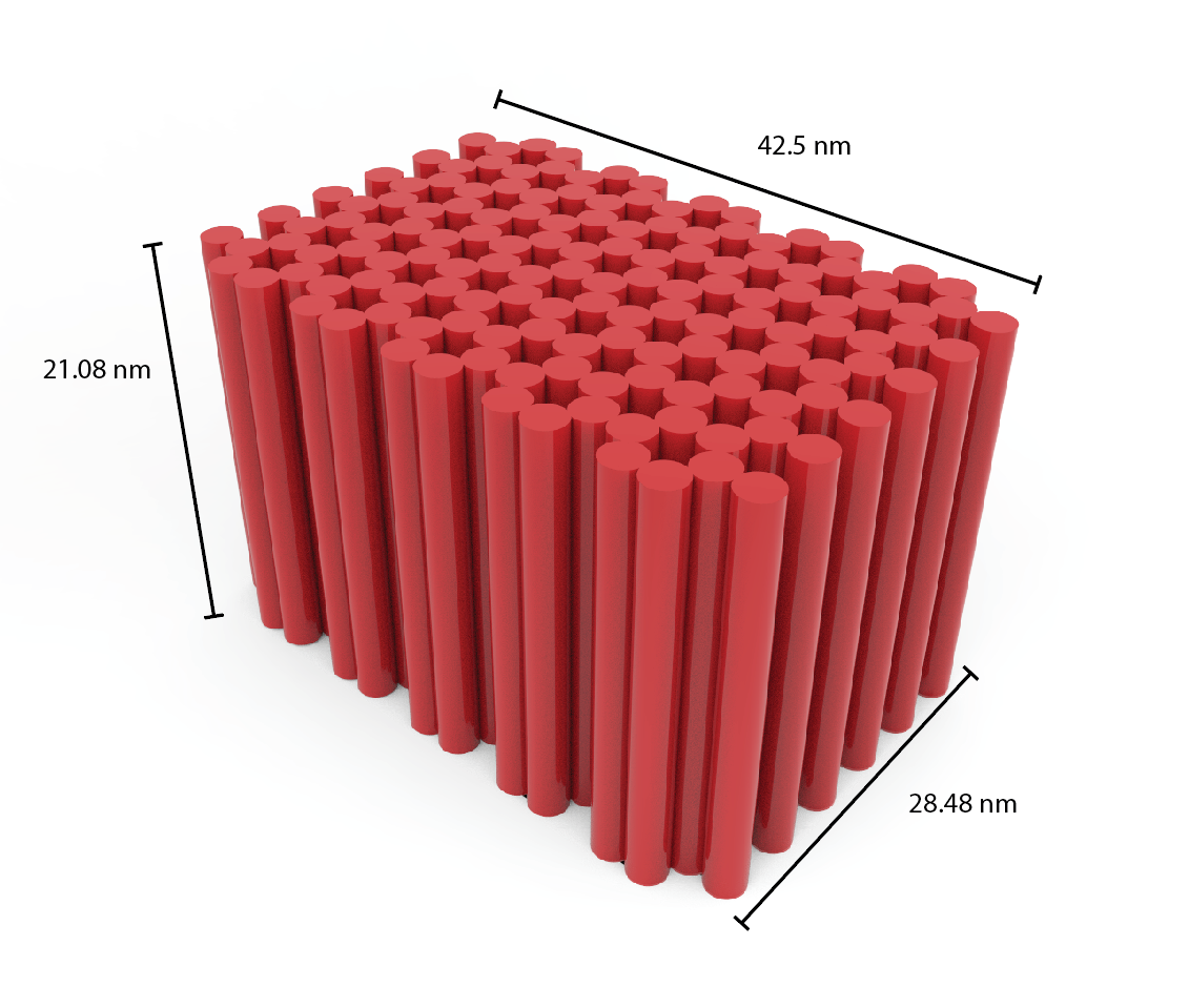
Figure 7: DNA Blockagon Dimensions

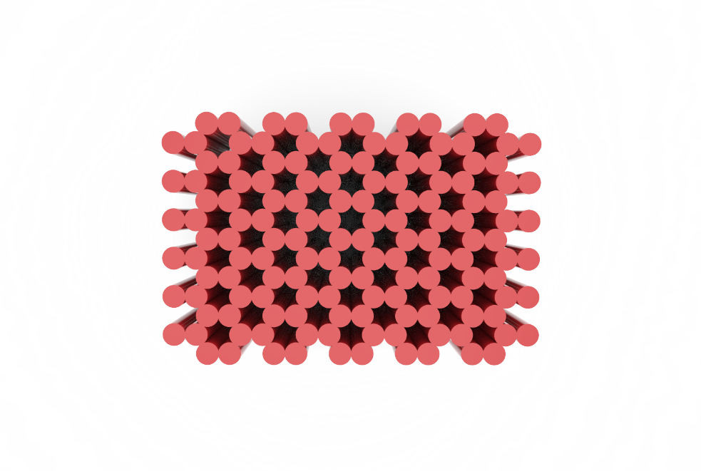
Figure 8: Blockagon Top View

By using Cadnano, we created the Blockagon structure using 115 helices. Helices were created in couplets so that the edges of the DNA backbone would line up, hence creating a flat surface.

The ends of certain DNA helices were chosen to be sites for binding to hexameric proteins. Using the distances of the hexamer C-terminuses (83.6Å), 6 neighbouring helices in a bundle with a 50Å diameter was determined to be the distribution with the closest diameter to the hexamer’s, hence this distribution decided our binding sites. We managed to fit 12 of these 6 helix bundles into our design as shown by the shaded circles in Figure 9.

Certain helices were also chosen to be sites for biotinylation so that they may be imaged for TIRF. Because DNA has a 5’ and a 3’ end, 8 sites for biotinylation were chosen (4 for each end). Even and odd numbered rods in Figure 9 have their 3’ and 5’ directed on the binding site side respectively. 3’ ends used for biotinylation are circled in black and 5’ ends used for biotinylation are circled in grey.

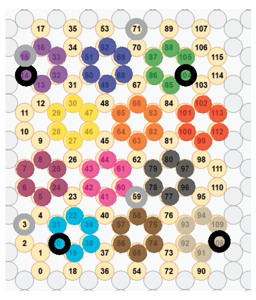
Figure 9: Cadnano Helix Arrangement

The Cadnano design in Figure 10 followed the following rules:

• Every helix is to have at least 2 or 3 crossovers with every neighbouring helix, of which 1 crossover is a backbone crossover
• Crossovers are to be kept at least 7 base pairs apart
• Must avoid kinetic traps
• Each strand is to have a seed region (14 base pair section) that is between smaller regions
• The shortest region in a strand cannot be between 2 longer regions
• If required to fulfil the above requirements, crossovers can use only a single strand rather than a double strand
• The absolute maximum length of a strand is 50 base pairs
• The absolute minimum length of a strand is 5 base pairs
• If there are strands shorter than 7 base pairs on the backbone edge, remove them
• If strands form loops within the structures, split them apart
• The helices chosen to be attachment sites for proteins were extended by 10 base pairs while remaining sites were extended by 5 thymine base pairs to prevent base stacking between structures
• Helices chosen to be sites for biotinylation were extended by 20 base pairs
• Binding site extensions were also planned to be attached to complimentary oligo strands so that extensions would be double stranded rather than single stranded. As we only possessed 5’ modified oligos, only the 3’ extensions could become double stranded.

Hence, we created the following versions of our structure:

• No extensions off the binding sites (passivated)
• Half the binding sites with extensions (even numbered helices activated)
• All binding sites with extensions (activated)

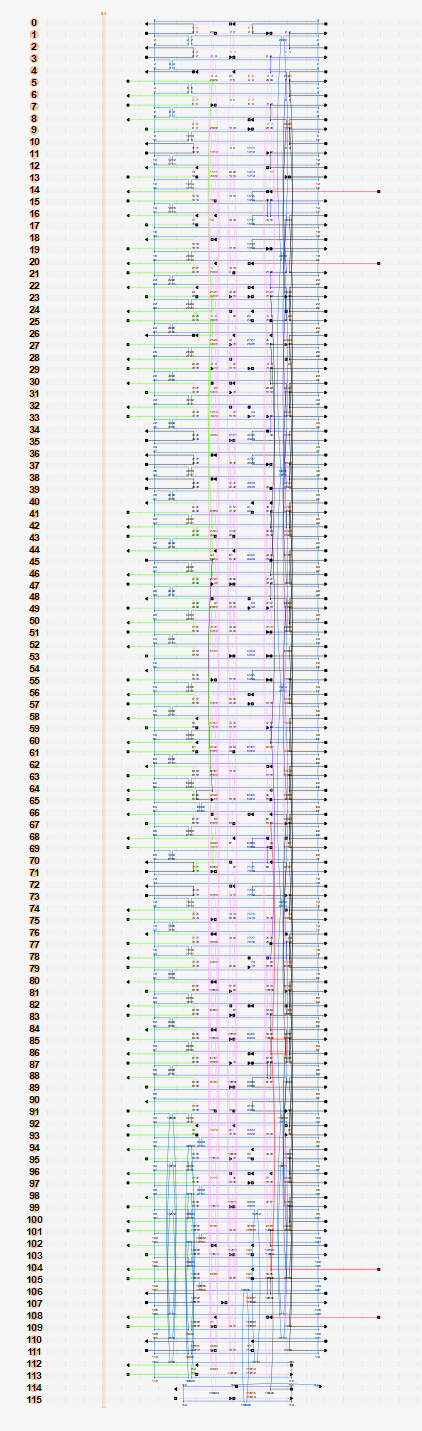
Figure 10: Cadnano Staple Routing

The following colours were used to highlight different types of strands:

• Green – binding strands
• Blue – m13a backbone strands
• Pink – internal strands
• Black – edge strands
• Red- biotinylation strands

DNA origami is formed by the process of annealing, where staple strands, backbone strands, buffer, water and salts (magnesium chloride) are mixed in solution and then subject to a cycle of rapid heating and slow cooling. Theoretically, each staple strand can fold a backbone strand, however in reality not all strands do. For this reason, staple strands are added in excess (usually in 5-fold excess). ⁵

The two most important factors for DNA origami formation are magnesium concentration and duration of the anneal.

Aqueous magnesium (Mg²⁺) creates a positively charged environment around the negative charge of the DNA, preventing them from the repelling each other due to electrostatic forces. The optimal concentration of magnesium depends on the complexity of the structure, and is determined by conducting a magnesium screen where the DNA origami is annealed in varying magnesium concentrations ⁶.  The results of our magnesium screen can be found here.

In the annealing process, there are two stages that the DNA is repeatedly subject to, a rapid heating and a slow cooling stage. The rapid heating denatures undesirable secondary structures, and the slow cool returns it to room temperature. By use of a thermocycler, varying time lengths are tested to find an ideal length of anneal. The results of our time screen can be found here.

The ideal conditions for synthesis were found to be 18mM of Magnesium, and 48 hours of anneal time.

The caDNAno Blockagon file was processed through CanDo software to produce the following images in Figure 11. They represent the side, front, and top views of the Blockagon respectively. These images clearly showed the structure as we intended it to be.

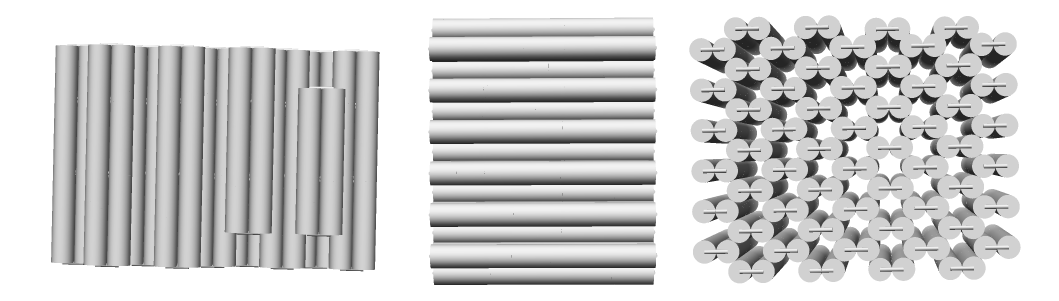
Figure 11: CanDo images of Blockagon.

The following movies were also outputted, showing relatively low instability , with a standard displacement of <0.8 nm (click to play).

Chimera X software was then used to produce the following PDB image (Figure 12). It visualises each strand in the DNA design, including the specific locations where crossovers occur.

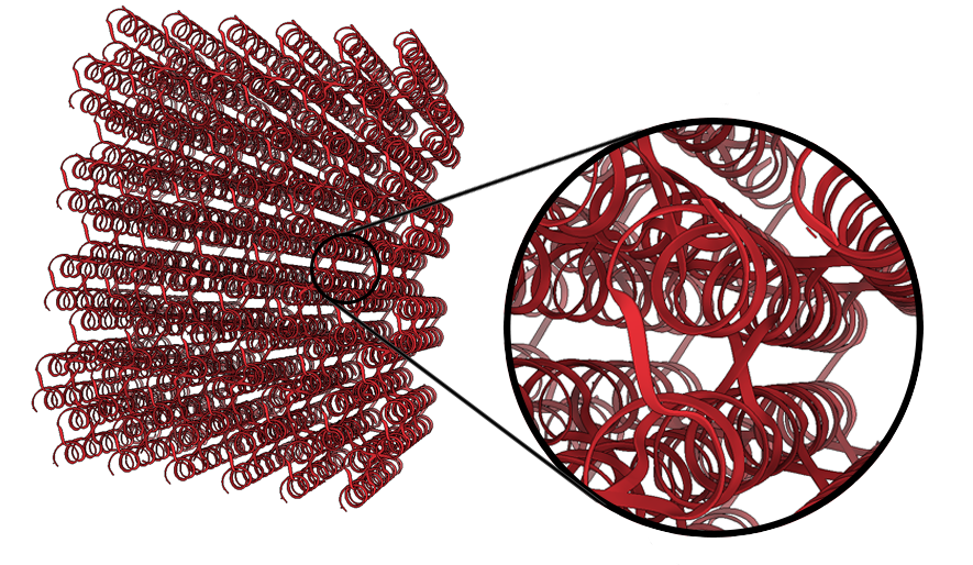
Figure 12: Blockagon PDB Image

A linear and ‘tennis racquet’ template DNA design were used for SPR experiments to measure the kinetics of protein conjugation to DNA.

The linear template is a 65-base pair sequence of DNA with a complementary 50-base pair sequence. The longer sequence has a 15 base pair overhang on the 5’ end (as shown in Figure 13) to allow for annealing to biotinylated DNA that forms the binding site for SPR and BLItz analytical instruments.

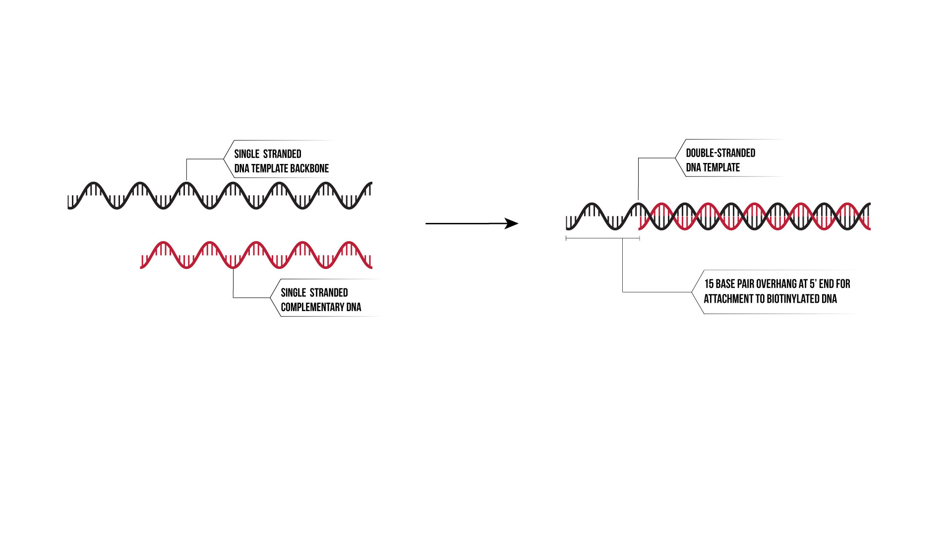
Figure 13: Linear Template Overhang

The ‘tennis racquet; design comprises of 6 domains for which proteins can bind to as shown in Figure 14. Between each domain there is also a single stranded poly-T domain. At the ‘handle’ of the racquet, there is a 15 base pair domain that closes the racquet up. Also attached to this is another 15 base pair domain that serves as an anchor domain that can attach to anchor strands on a surface such as an SPR chip or a TIRF microscope slide.

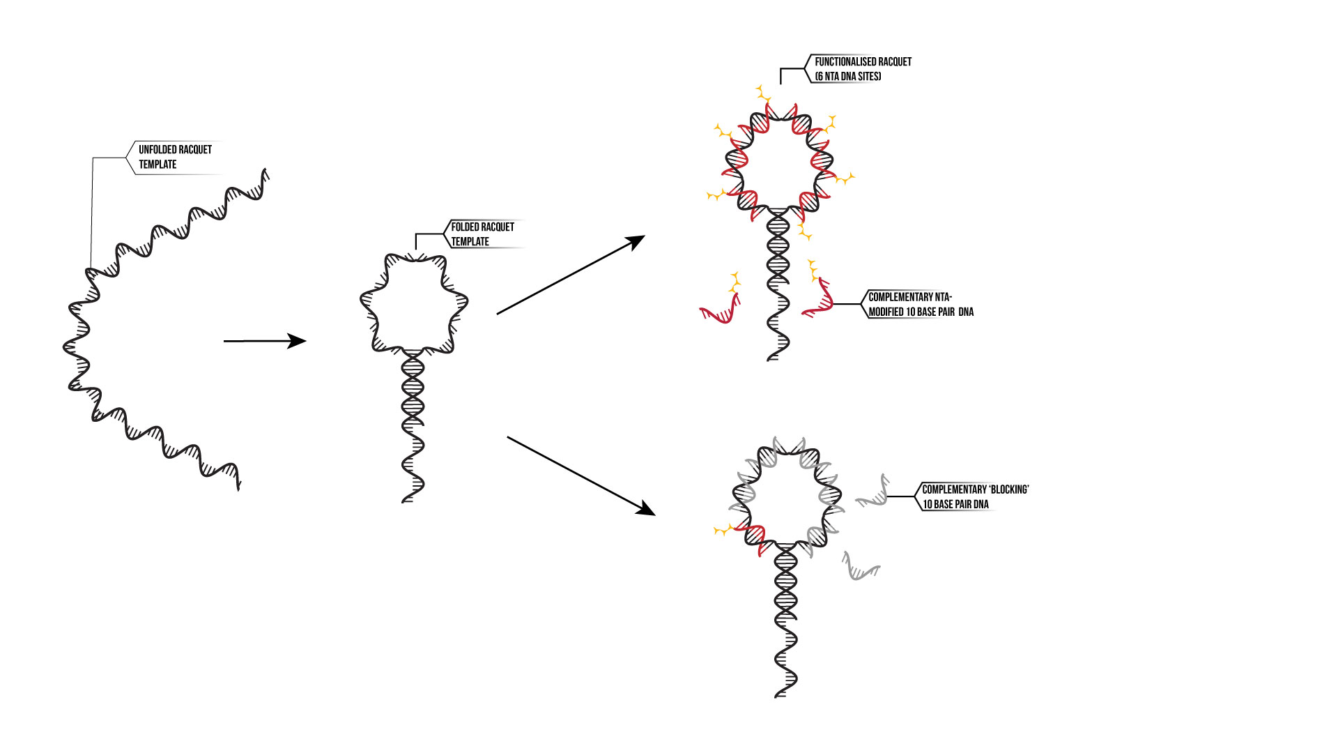
Figure 14: Tennis Racquet Template

Further information on how these designs were used can be found here.

Our DNA origami structure successfully formed with 12 potential positions for hexameric proteins to attach to. The structure was suitably stable and able to form at a consistent size as shown by EM images. We were also able to create our desired single stranded DNA for SPR experimentation.

In future, we would like to further characterise our DNA origami structure so that we have a comparison between the dimensions of the formed DNA and the intended dimensions in the design. We would also like to create an extensive analysis on the size distribution of our structure in the various conditions that we synthesized it in.

Furthermore, we would like to create more variations in the binding sites of our structure. By having a variety of allocations of the hexamer binding sites, we may conduct more experiments that analyse the hexamer binding to the origami and their effects on other bound hexamers.

Ordering

DNA was ordered from Integrated DNA Technologies

• V-well (shallow) 96 well plate for edge staples, internal staples, binding staples.
• Single tubes for biotinylating extensions
• Normalised to highest amount
• Standard desalting purification
• Dry shipping

Resuspension

1. Spin down plates/tubes at 4000 rpm, 20°c for 10min to dislodge the pellet from the top or sides. Resuspend the pellet in water up to 1uM for internal, edge, and binding staples. Resuspend up to 10uM for biotinylating extensions
2. Seal the plate very well with a foil cover and store -20°

Staple Mixes

1. Spin down plates/tubes at 4000 rpm, 20°c for 10min
2. Pipette 2uL of each staple into its respective tube

Synthesis

• Magnesium screen: 0-30 mM Mg should be screened to find optimal conditions for synthesis. 3mM increments: 0, 3, 6, 9, 12, 15, 18, 21, 24, 27, 30 mM over 37hr anneal time.
• Time screen: Synthesis times should be screened to find shortest time in which you can make well-formed origami. The more complex the structure the more time needed for synthesis.

Total Reaction Volume (uL)	15.00
Reactants	Reaction Concentration (nM)	Stock Concentration (uM)	Volume to Pipette 1x reaction (uL)
m13	20.00	0.45	0.67
General staple mix (internal and edge staples)	100.00	1.00	1.50
Binding staples	100.00	1.00	1.50
Biotinylation extensions	100.00	10.00	0.15
Buffer (1mM EDTA and 5mM Tris)			1.50
Total Volume			5.32
Mg + H2O			9.68
Total (uL)			15.00

Magnesium Reaction Concentration (mM)	100mM MgCl2 (uL)	Water (uL)
0	0	9.68
3	0.45	9.23
6	0.9	8.78
9	1.35	8.33
12	1.8	7.88
15	2.25	7.43
18	2.7	6.98
21	3.15	6.53
24	3.6	6.08
27	4.05	5.63
30	4.5	5.18

Temperature	24 hr anneal	36 hr anneal	37hr anneal	48 hr anneal	71 hr anneal
65°C	15min	15min	15min	15min	15min
65-60°C	1 min/-0.1°	1 min/-0.1°	1 min/-0.1°	1 min/-0.1°	1 min/-0.1°
60-40°C	4 min/-0.1°	6 min/-0.1°	10 min/-0.1°	8 min/-0.1°	12 min/-0.1°
40-25°C	4 min/-0.1°	6 min/-0.1°	1 min/-0.1°	8 min/-0.1°	12 min/-0.1°
storage	RT	RT	RT	RT	RT

Purification - Agarose Gel Electrophoresis

1. Gel composed of 100mL of buffer (90mL water, 9mL 0.5 TBE, 1mL 1M MgCl₂), 2g agarose, and 5uL of gelred dye. Before dye is added the buffer is microwaved for 2 minutes to dissolve the agarose
2. Solution is poured into a gel mould with a lane comb within
3. Gel immersed in 300mL of buffer
4. Samples, a 1kb ladder are loaded into the lanes
5. The 2 controls used are the staple general mix and m13
6. Run 70V through the gel for 2 hours
7. Cut out desired bands under UV illumination and insert into freeze and squeeze tubes
8. Keep tubes in -20°c for 5 min, centrifuge at 13000 rpm for 3 min at room temperature
9. Remove excess material
10. DNA collected in the dolphin tube ready to use.

1. Folding DNA to create nanoscale shapes and patterns. Rothemund, P W K. s.l.: Nature, 2006, Vol. 440.
2. Self-assembly of DNA into nanoscale three-dimensional shapes. Douglas, S M, et al. 8, s.l.: Nature, 2009, Vol. 459.
3. A primer to scaffolded DNA origami. Castro, C E, et al. 3, s.l.: Perspective, 2011, Vol. 8.
4. [Online] 2011. https://eurofinsgenomics.jp/media/48523/product-sheet-single-stranded-scaffold-dna-type-7249-m1-10.pdf.
5. Magnesium-free self-assembly of multi-layer DNA objects . Martin, T G and Dietz, H. s.l.: Nature Communications, 2012.
6. Rothemund, P W K. Design of DNA origami. s.l.: California Insitute of Technology.