Introduction
We are artificially constructing the HIV capsid by binding HIV-1capsid subunits in defined configurations to DNA templates. This increases the local concentration of protein and allows us to observe the rate of assembly of subunits into pentamers and hexamers. Here, we model this process mathematically to extract the fundamental rate constants that govern this process of self-assembly from experimental data.
The problem itself arises due to the difficulty in controlling and observing the formation of pentamer and hexamer structures from the native capsid protein. By facilitating the self-assembly of the capsid proteins with a DNA scaffold in vitro, we can better understand the spontaneous formation of the HIV capsid in vivo.
Observations of the binding events largely took place through Surface Plasmon Resonance, Biolayer Interferometry and gel band-shift experimentation. In addition, TIRF was investigated as an avenue to visualise single-molecule interactions. An understanding of the particular protein, any conjugation chemistry relevant to the experimental design, and the geometry of the origami structure, allows a description and quantitative model to be developed explaining the assembly of proteins in a particular system. To that end, modelling may be used to calculate information useful to the fundamental understanding of the capsid structure.
Aims
Using the mathematical model developed, we aimed to quantify the interaction strength of capsid proteins as they form pentamers and hexamers. Subsequently, we wanted to quantify the stability of pentamer and hexamer structures formed from capsid proteins in order to evaluate the conditions within which the capsid forms in vivo.
Additionally, we planned to develop a working model for aggregation of capsid proteins into pentamer and hexamer forms. By doing so, we have established an experimental design suited to test and monitor self-assembly of proteins more generally.
Methodology
The problem of setting up a model for the aggregation of proteins has been approached through the use of ordinary differential equations (ODEs). ODEs describe how a system, or a particular state, changes over time. Put simply, they are a language by which we can precisely define the evolution of a system.
ODEs are often coupled. This means that the change in a particular state over time is dependent on one, or several other states, which too change with time. In order to solve such coupled ODEs, a complete set of equations is necessary. Programs such as MatLab can then be used to output numerical solutions. The drawback of this method is that all states must be predetermined; the model does not yet account for more complex aggregations, or pathways in addition to those described below.
In kinetic experimentation, we used a ‘racquet’ DNA construct (Figure 1). To learn more about this structure, check out our DNA design. Through modelling we aimed to discover how the proteins were binding to these racquets, and the paths through which they form pentamers and hexamers.
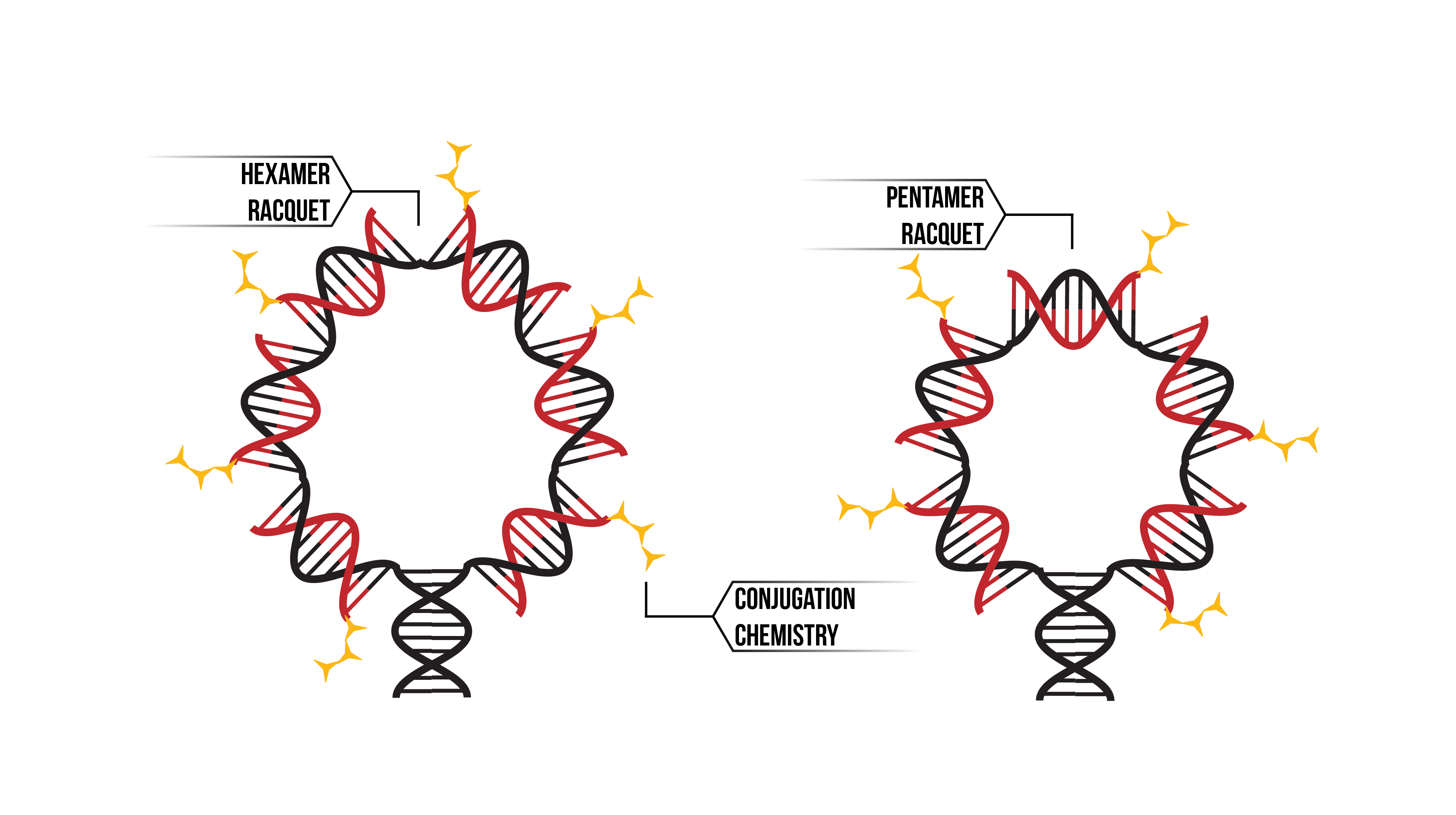
Figure 1: Through the use of conjugation chemistry (Yellow), we were able to bind our proteins to a DNA template. The racquet template was built in two sizes; as a hexamer (Left) and as the pentamer (Right). Functionalised DNA (Red) was annealed onto the template backbone (Black)
Experimental limitations
SPR and BLItz detect small changes in mass over time. Thus, many ‘different’ states under this model will be measured as identical and indistinguishable. Experiments must either be carefully designed to test particular interactions and exclude unwanted binding events, or data must be deliberately analysed in consideration of the complex binding phenomena occurring at the nano-scale. Alternatively, single molecule experimentation may serve to increase the resolution of our binding experiments, overcoming inherent ambiguity in bulk measurements.
Pentamer and hexamer formation
We can visualise the binding pathways for the formation of pentamer and hexamer protein aggregates by creating a branching tree (Figure 2 and 3 respectively).
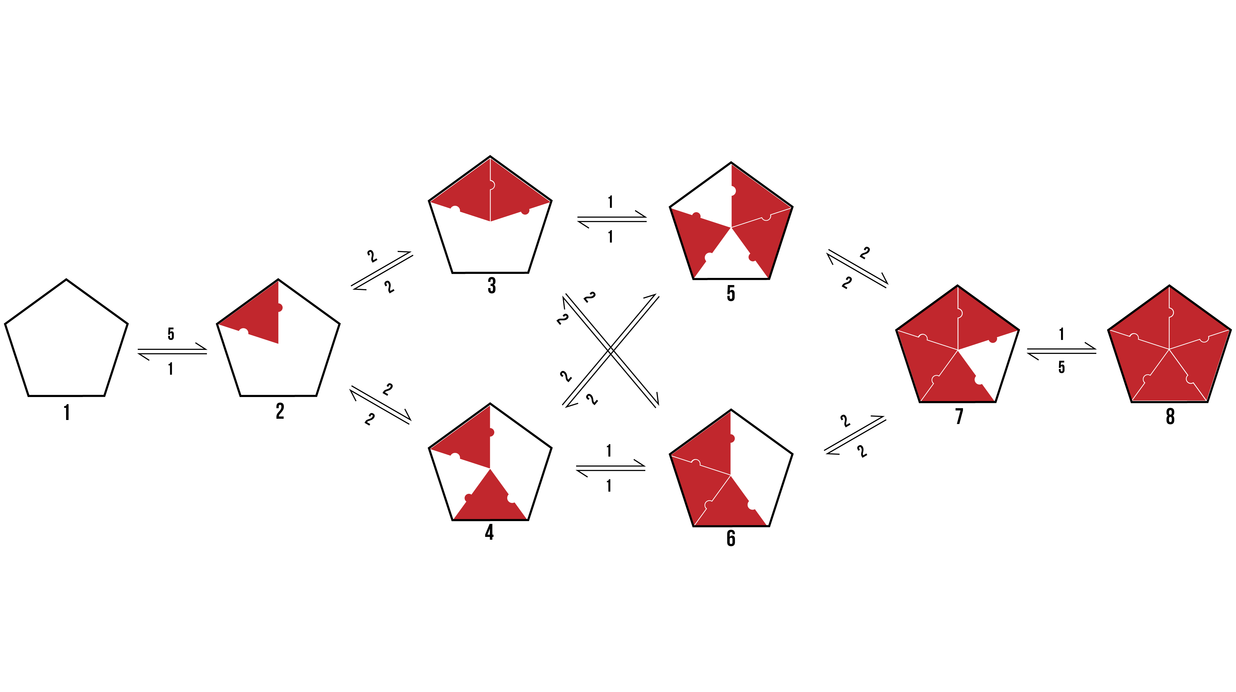
Figure 2: The possible binding pathway of proteins (Red) onto a pentamer racquet (Black). The numbers represent how many possible transitions there are between two states.

Figure 3: The possible binding pathway of proteins (Red) onto a hexamer racquet (Black. The numbers represent how many possible transitions there are between two states.
From the above pathways, we can see the formation of pentamers and hexamers from an empty DNA template. It assumes binding events are discrete, and rotationally symmetrical. The number allocated to each binding event is dependent on the number of variations a particular transition encompasses which would still reach the same final state.
When looking to the above binding pathways, each step may be characterised in one of three ways. Firstly, a protein may bind to a template at a location that has neither adjacent sides occupied. Secondly, a protein may bind to a template at a location that has one adjacent side occupied. Thirdly, a protein may bind to a template at a location that has both adjacent sides occupied. Thus, we can break the problem down into a zero-neighbour, and one-neighbour, and a two-neighbour case.
Mass action
Protein self-assembly will be made up of binding and un-binding events. In order to mathematically describe these events, in the context of differential equations, it is important to utilise the mass action principle. This principle states that a binding event is dependent on the concentration of the monomers which are involved in binding. Conversely, an un-binding event is independent of the concentration of monomers.
Assumptions
As in all models, it is crucial to outline the assumptions made in order to assess the strength of the theoretical description of a physical system. The key assumptions made are outlined below.
- Identical, concentration-relevant interactions
When considering the model developed, it is assumed that there are two discrete binding interactions that may occur. Firstly, a protein may bind to (or un-bind from) the racquet template. Rate constants define the likelihood and speed with which a particular transition occurs. In the binding/un-binding of a protein to the racquet template, we use rate constants `k_+^T` and `k_-^T`.
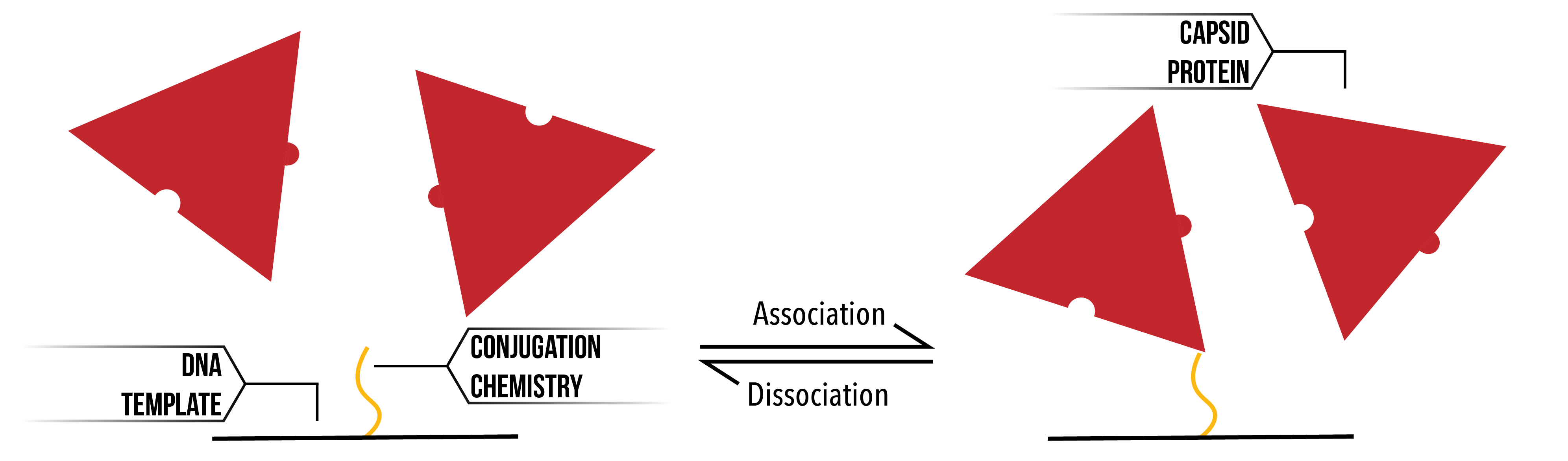
Figure 4: Proteins (Red) binding and unbinding from a section of the racquet template (Black) through conjugation chemistry (Yellow).
Secondly, the protein may bind to another protein in the system. This interaction will have associated rate constants `k_+^P` and `k_-^P`.

Figure 5: Proteins (Red) binding to each other whilst attached to the DNA template (Black).
As discussed, association is concentration dependant, whilst disassociation is concentration independent.
- Two-neighbours
The assembly of proteins into pentamer and hexamer forms can be broken down into a series of zero, one and two-neighbour cases. The assumption is supported by the geometry of the DNA structure, which is hexameric/pentameric in nature.
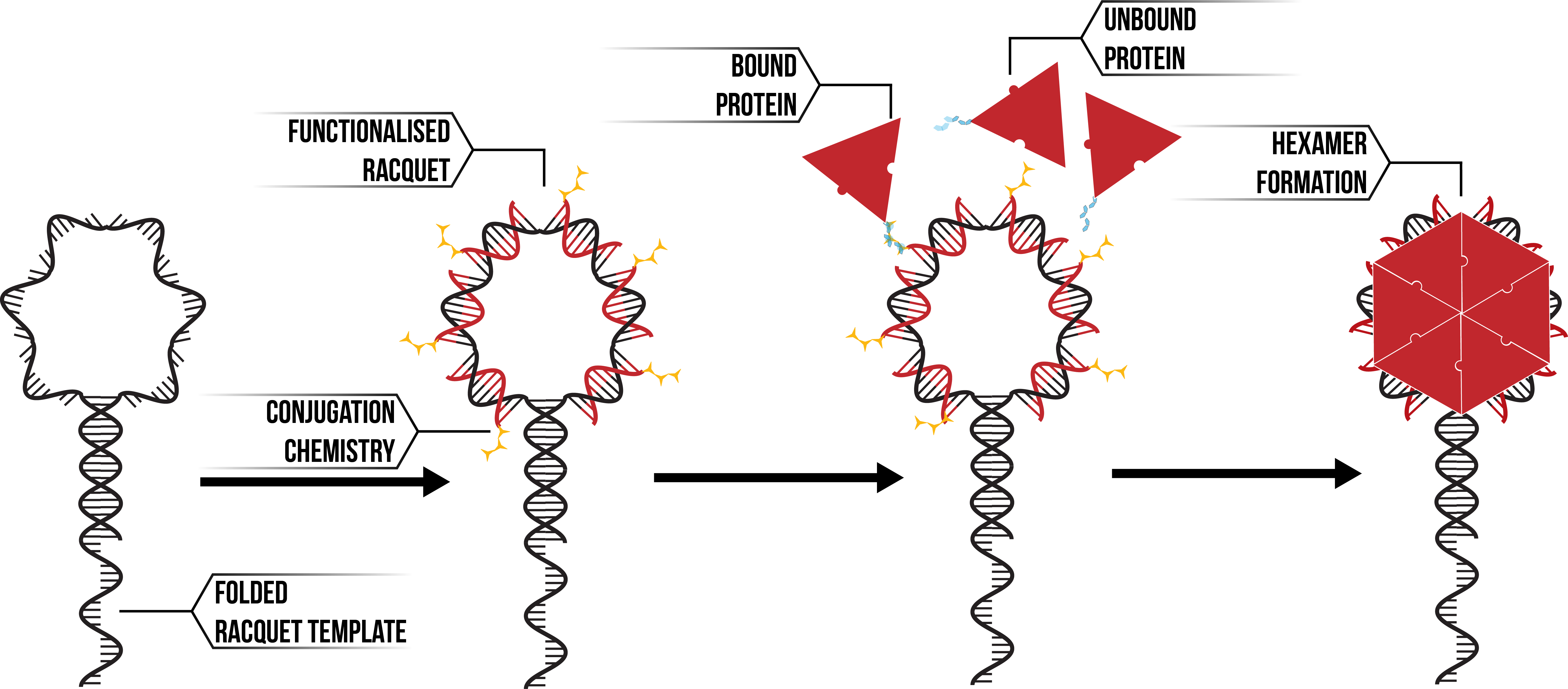
Figure 6: Hexameric DNA racquet (Black) annealing with functionalised DNA (Red). Proteins (Red) bind to the template through conjugation chemistry (Yellow) to form aggregates such as hexamers.
However, as the backbone of the racquet template consists of single-stranded DNA, it is possible that the inherent flexibility leads to a breakdown in this assumption. Instead, proteins may be able to bind to other subunits opposite it on a particular template. This may be remedied if the `k_-^P` is very high (and thus proteins regularly un-bind), or if the distance between the subunits decreases the likelihood of a binding event to occur.
Additionally, research has begun on developing a stronger, more rigid racquet structure. However, we were unable to complete experiments using this new racquet due to time constraints.
- Effective concentration
As already described, association is dependent on the concentration of monomers. However, by increasing the local concentration of proteins in the vicinity of the template through protein-template binding events, the relevant concentration is no longer the easily identified solution concentration (`m_f`). Instead, an ‘effective’ concentration (`m_f`) must be established, calculated with reference to the geometry of the system and the length of any conjugation chemistry.

Figure 7: Two possible pathways through which Protein-Protein binding may occur. Evidently, the concentration in Panel B) is higher than in Panel A). Due to the increase in local concentration, the second case is more likely than the first. As such, we introduce the term ‘effective concentration’ to quantify this increase in probability.
Naming Conventions
To remove ambiguity in our descriptions, a relevant naming convention must be established. Each step (ie. Association and dissociation in the context of a zero, one or two-neighbour solution) involves a single protein changing states. Thus, the convention relates to the possible binding combinations of such a protein. Each template-protein binding configuration is characterised by the descriptor `S_{n, t, p}`. The first term, `n` , describes how many proteins are attached to the template binding site. The second term, `t` , describes whether the ‘additional’ protein is attached to the template. The final term, `p` , describes whether the additional protein is attached to other surrounding proteins.
Results: Zero, one and two-neighbour Solutions
By breaking down the formation of pentamers and hexamers into zero, one and two-neighbour solutions, the process of analysis simplifies greatly.
Zero-neighbour case
The zero-neighbour case involves a protein binding to a location of the template that has neither adjacent sides occupied. From the two-neighbour assumption, we can simplify the depiction of these states. Rather than represent the racquet as hexameric, we can represent the template as a platform with three binding sites.
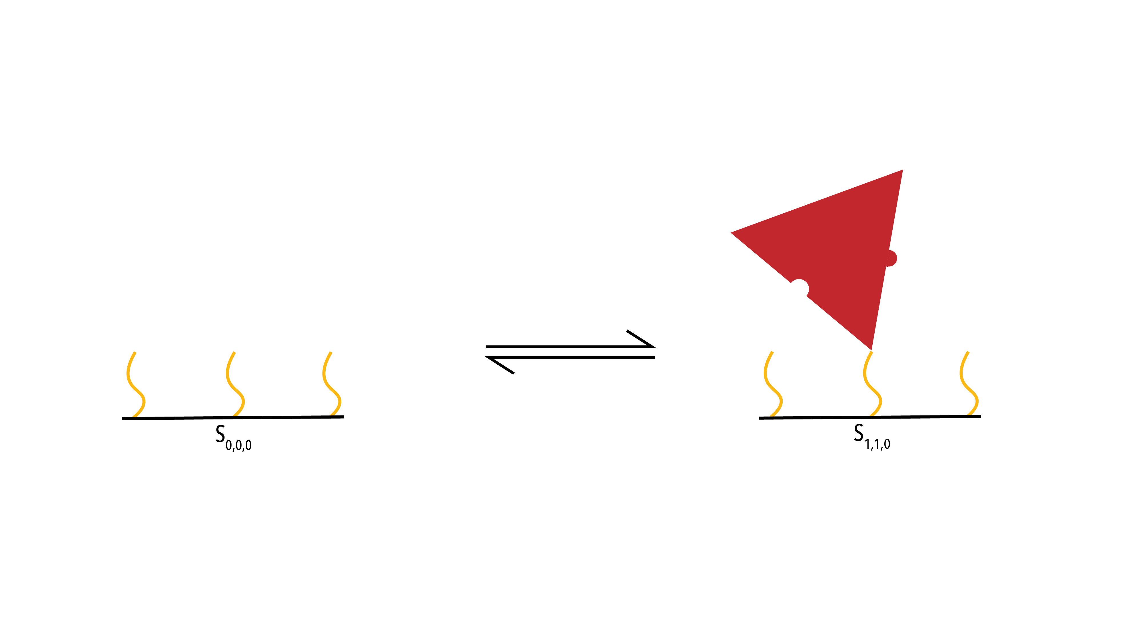
Figure 8: Protein (Red) binding to the racquet backbone (Black) through conjugation chemistry (Yellow)
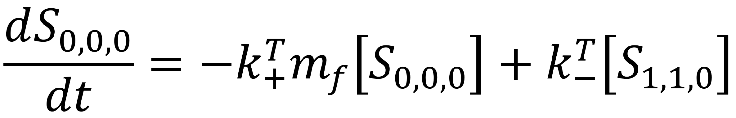
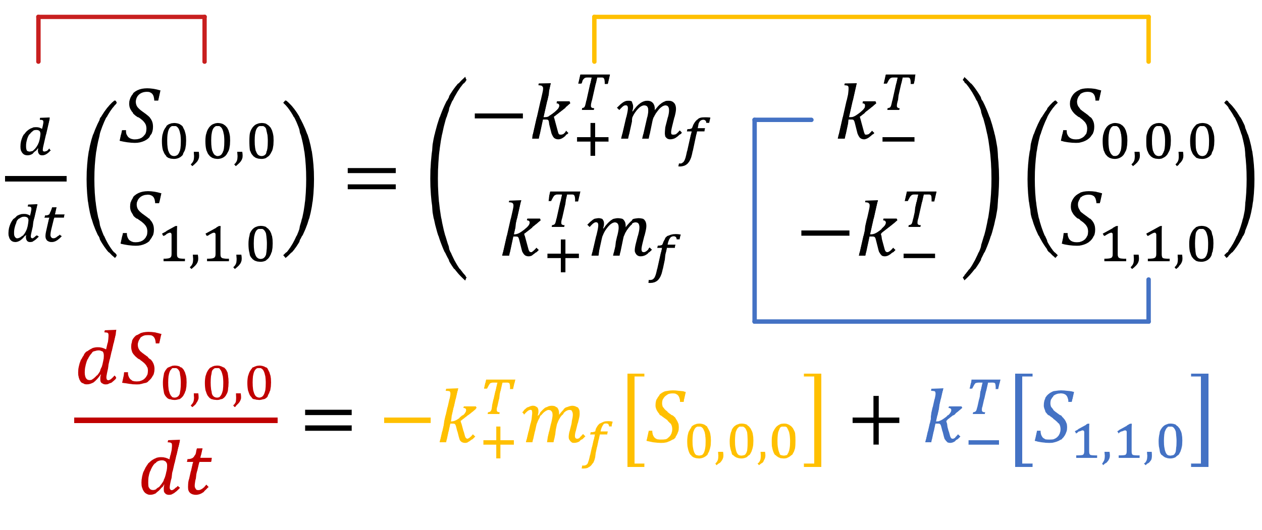
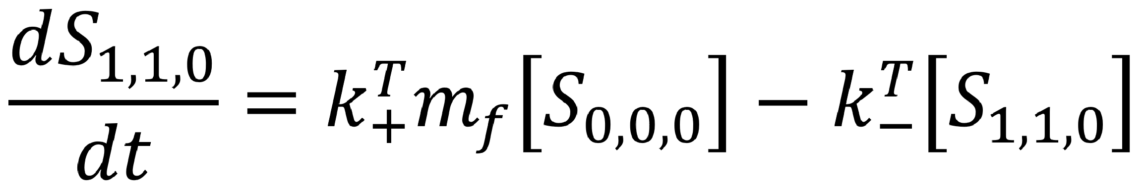
The above diagram displays all possible states in the zero-neighbour case. We can use the mass action principle to determine the rate of change of the state `S_{0,0,0}`. First, we look to the arrow travelling from the initial state (`S_{0,0,0}`) to the final state (`S_{1,1,0}`). This is the binding event of a protein to the template, and so it has associated rate constant `k_+^T`. As it is a binding event, it is concentration dependent. Thus, we multiple the rate constant by the concentration of proteins, and the concentration of empty template binding site (the two things involved in the interaction).
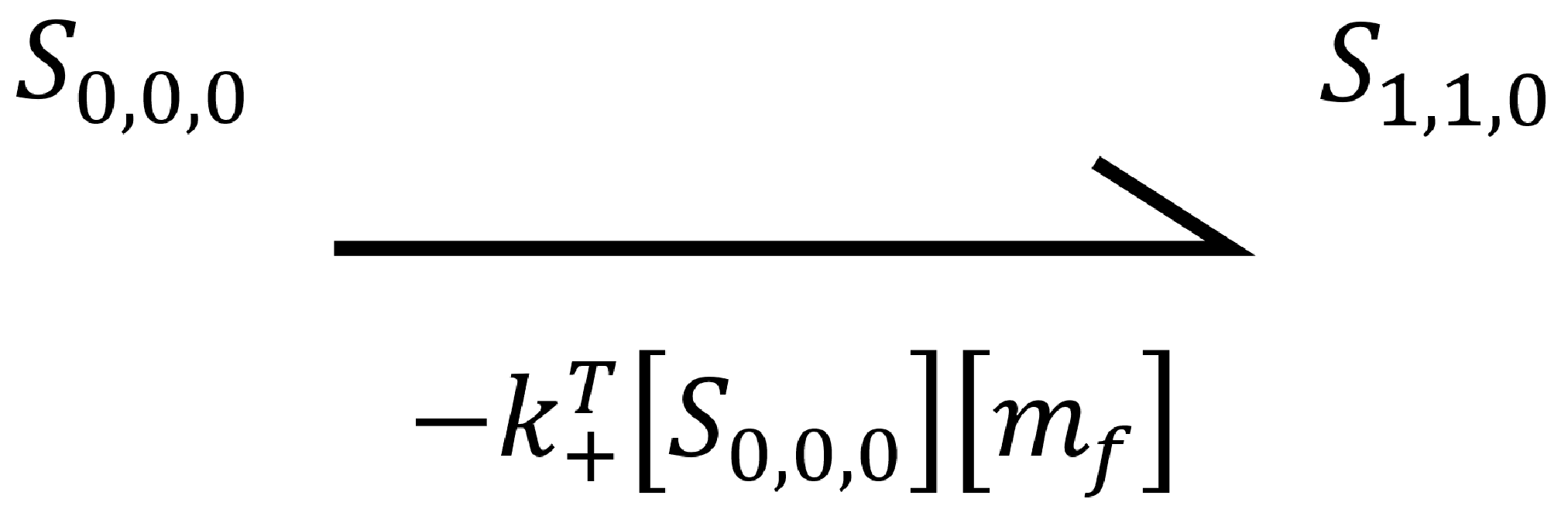
The minus sign is an indication of the directionality of the transition. When the first state transitions to the second, its concentration will decrease.
Secondly, we look to the arrow travelling from the final state (`S_{1,1,0}`) to the initial state (`S_{0,0,0}`). This is the unbinding event of a protein to the template, and so has associated rate constant `k_-^T`. As it is an unbinding event, the protein concentration is no longer relevant.
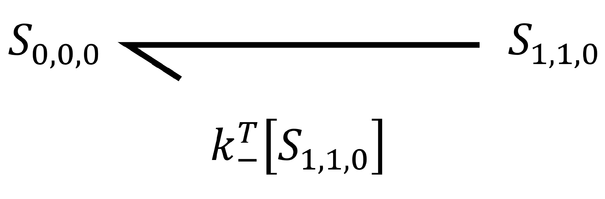
This transition is positive, as when the second state transitions back to the first, the concentration of the first state will increase. Overall, we can describe the rate of change of the first state as an ordinary differential equation.
Similarly, we can identify the differential equation describing the rate of change of the second state.

An important check is whether the two rates add to zero. As the only allowed transitions have been pre-determined, the ‘net’ rate of change (ie. `(dS_{0,0,0})/dt+(dS_{1,1,0})/dt`) should be equal to zero.
We may represent this system of equations more easily in a matrix form.
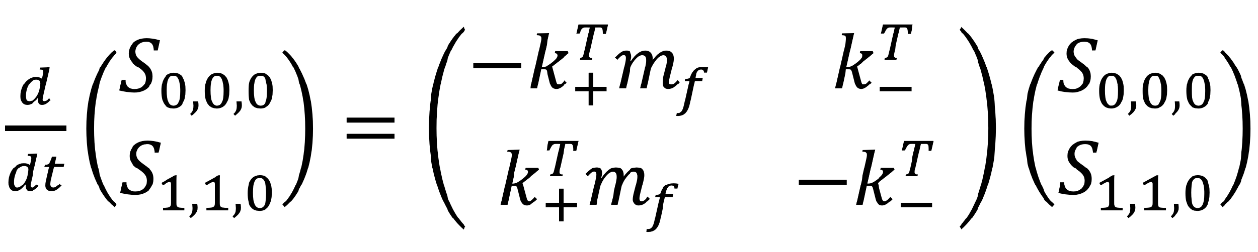
Matrixes are a simply way to represent multiple equations containing the same or similar variables. They also allows us to see whether there are any nice patterns forming in the mathematics!
Generally, solutions to complex sets of equations such as these have a numerical solution. A numerical solution is an approximation; programs are able to ‘fit’ a graph or a function to a set of equations as best as it can. However, this particular set of equations have an exact solution. Exact solutions are mathematically exact solutions to differential equations.
The exact solutions to the zero-neighbour case are
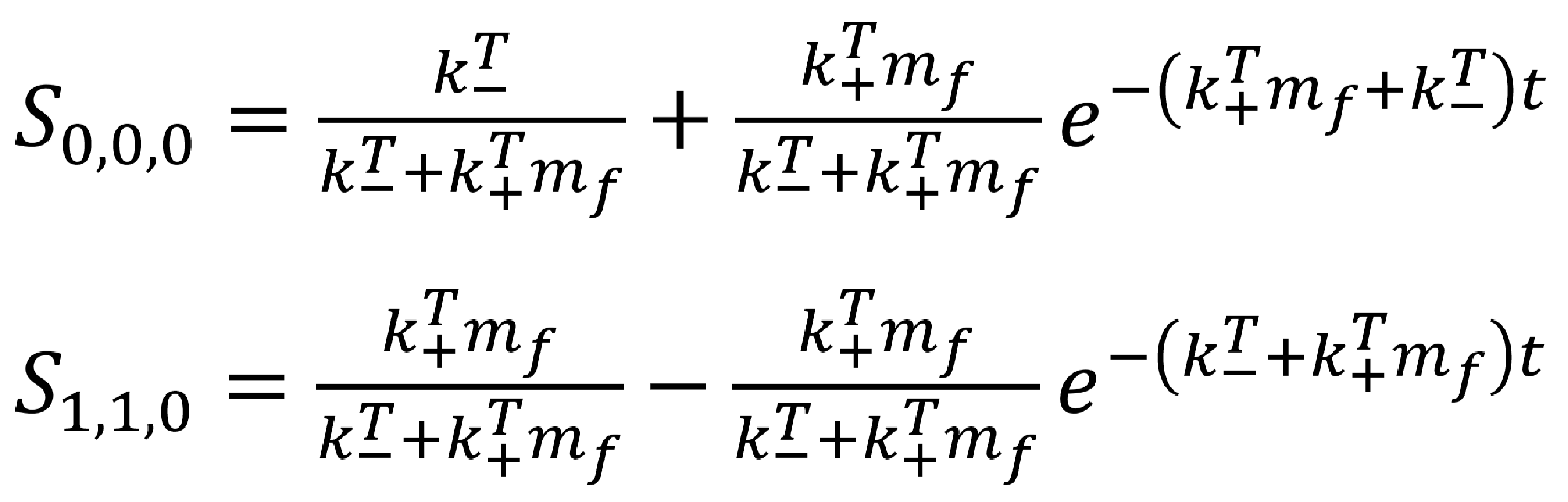
We can plot these curves for a number of binding and un-binding constants. By comparing these theoretical graphs to any experimental results obtained, we can quantify the real binding constants associated with our capsid proteins!
| `m_f=20×10^(-6) M` | `k_+^T=10×10^5` | `k_+^T=10×10^3` |
| `k_-^T=10×10^(-3)` | Solution 1 | Solution 2 |
| `k_-^T=10×10^(-2)` | Solution 3 | Solution 4 |
Hover over the cells above to see the corresponding solution appear below.
One-Neighbour Case
The one-neighbour case involves a protein binding to a location on the template that has one adjacent side occupied.
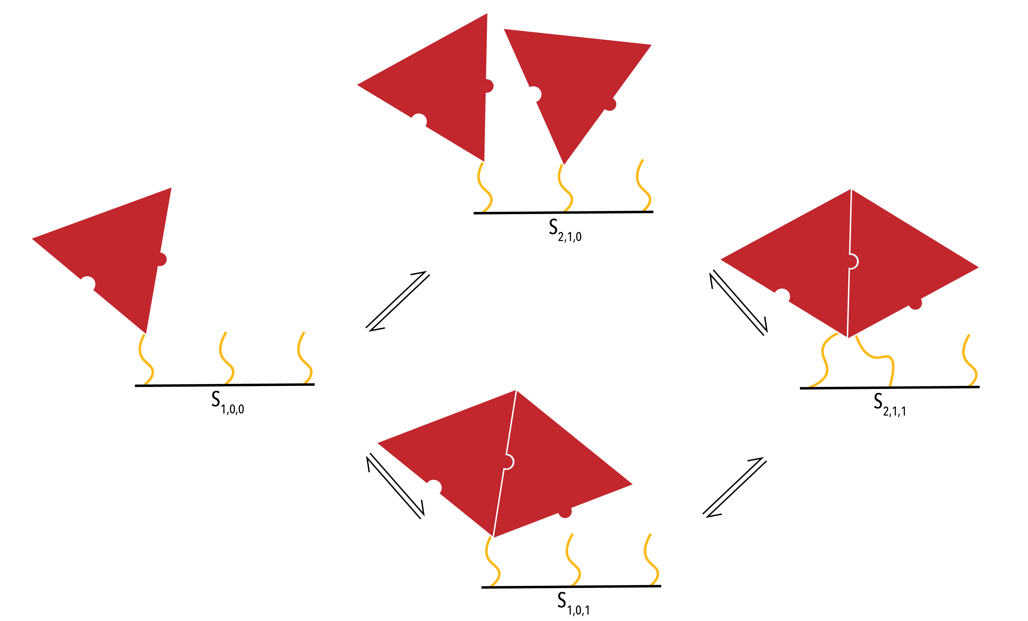
Figure 9: Close up of the binding pathways in the one-neighbour case. The binding sites (yellow) physically represent the conjugation chemistry on the DNA racquets.
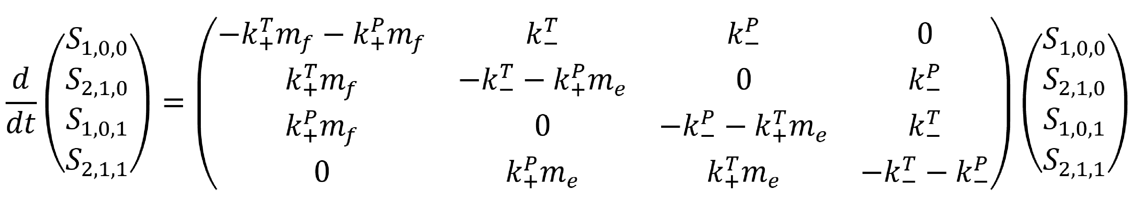
The above diagram displays all possible states in the one-neighbour case. Again, we can use physical principles to derive a set of ordinary differential equations to describe the system.
Two-Neighbour Case
In the two- neighbour case, there are a number of symmetrical states. For example, the following two states are identical.

Figure 10: Two symmetrical states which, for the purpose of this model, will be treated as identical
However, a transition to the above state will be twice as likely, as there are two possible avenues through which to arrive at it. As such, the pathway relevant to any transition to this state has the number ‘2’ attached to it. This coefficient is reflected in the differential equations derived for this system.
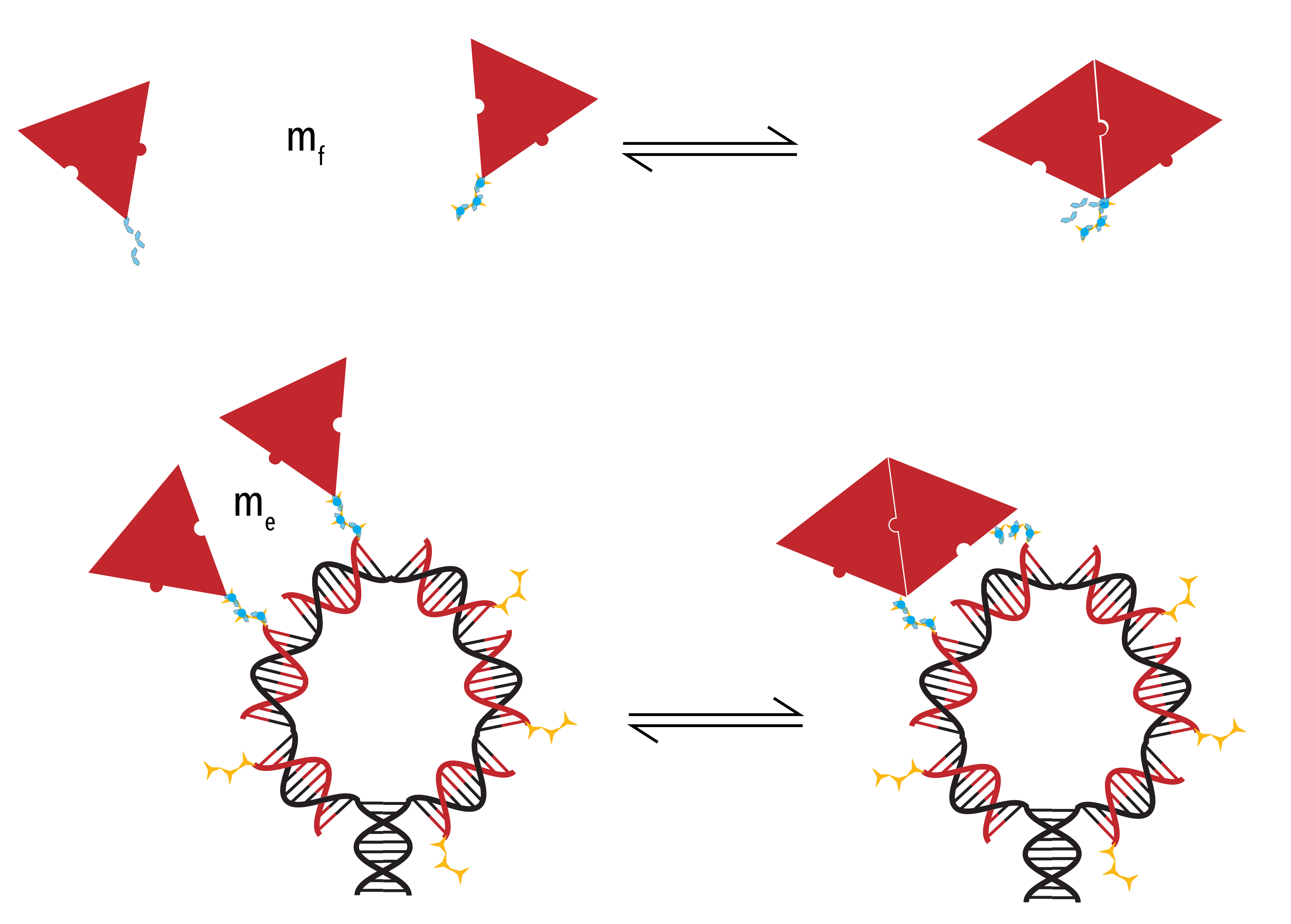
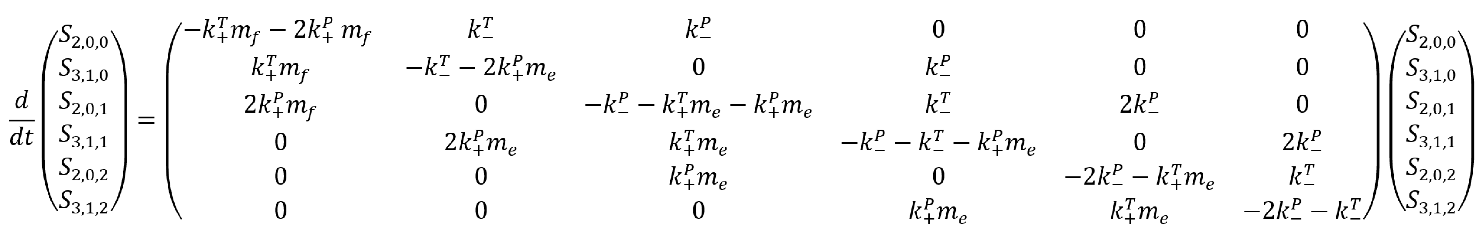
Figure 11: The possible binding pathways in the two-neighbour case. The three binding sites represent adjacent strings of conjugation chemistry onto which the proteins may bind.
The differential equations describing this system are:
Extracting rate constants
The above description of binding and unbinding events are useful as they allow as to extract ‘virtual’ rate constants for the rate of subunit binding to a template with zero, one or two occupied neighbouring sites. As will be seen, this data would allow us to accurately describe the process by which pentamer and hexamer protein structures are formed.
Where Surface Plasmon Resonance data is taken, we can use a number of methods to extract the relevant rate constants. We will look at only one of them here.
Recall our zero-neighbour ordinary differential equation,
This equation describes the rate of change of a protein bound to the template. If the reaction is assumed the be one-to-one (eg. by using a racquet scaffold with only one functionalised site), we can manipulate this relationship to get to
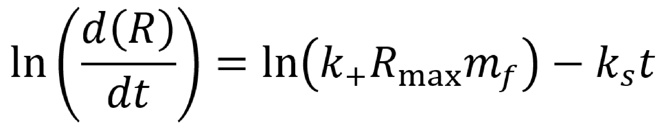
Where `R` are the response units of the SPR output, `R_max` is the maximum change in response units during the kinetic experiment, and `k_s=k_+ m_f+k_-`.
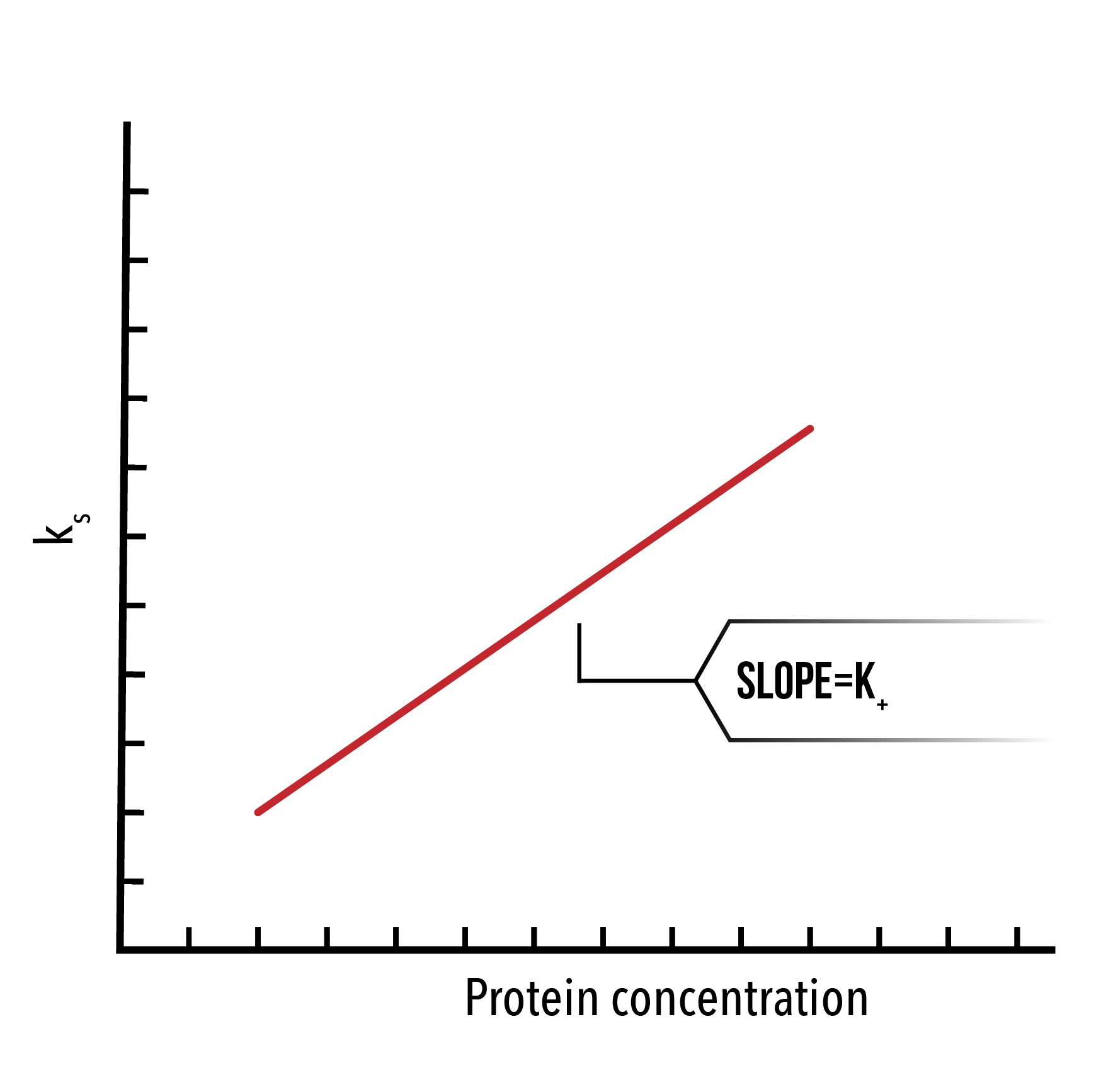
Next, we plot `ln(d(R)/dt)` against time for a number of protein concentrations. By selecting the linear portion of such a graph, we can extract and plot `k_s` against the protein concentration, and thus extract `k_+` as the slope.
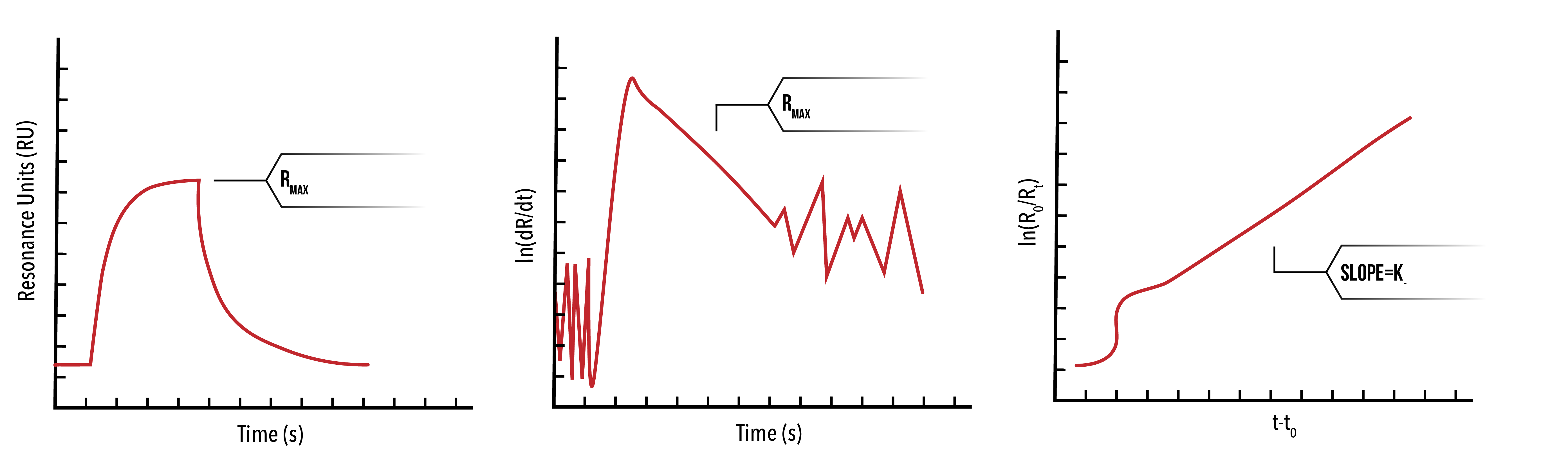
We may also extract the dissociation constant using the unbinding phase of the SPR data. To do this, we plot `ln(R_0/R_t )` against `(t-t_0)`, where `R_0` is the response units at `t_0`. The resulting linear function will have slope `k_-`.
Ideally, when dealing with cases more complex than the zero-neighbour case (ie. Where multiple rate constants may be variable), we will have previously extracted solutions to the most simple case. From there, we can use the methodology above to produce a ‘virtual’ rate constant for the particular experiment. By factoring in the relevant binding constants that are involved in the overall ‘virtual’ rate constant we may be able to identify values for higher neighbour solutions.
Alternatively, we may run a MatLab simulation designed to alter the various input rate constants, and fit the output curve to experimental data. By scanning through each a range for each rate constant, and plotting the constant versus the root mean square of the discrepancy between the experimental and theoretical data, we can find a global minima that best fits the data set. Thus, we can identify the best-suited rate constant for a particular experiment. By repeating this process for multiple concentrations, and several experimental designs, we can accurately extract the rate constants sought.
Results: Pentamer and hexamer formation
With an understanding of the zero, one and two-neighbour binding solutions, we can begin to approach the problem of pentamer and hexamer formation. By breaking down each binding/unbinding event into a neighbour solution, we can write out the equations governing self-assembly in a similar manner to those equations derived above.
In the equations derived below, `k_(a->b)` indicates the rate constant relevant to a particular neighbour solution.
|
Rate constant |
Neighbour solution |
Binding/un-binding |
| `k_(1→0)` |
Zero-neighbour |
Binding |
| `k_(0→1)` |
Zero-neighbour |
Un-binding |
| `k_(1→2)` |
One-neighbour |
Binding |
| `k_(2→1)` |
One-neighbour |
Un-binding |
| `k_(2→3)` |
Two-neighbours |
Binding |
| `k_(3→2)` |
Two-neighbours |
Un-binding |
Pentamer

`\frac{d[1]}{dt}=-5k_{0\rightarrow 1}m[1]+k_{1\rightarrow 0}[2]`
`\frac{d[2]}{dt}=-k_{1\rightarrow 0}[2]+5k_{0\rightarrow 1}m[1]-2k_{1\rightarrow 2}m[2]+2k_{2\rightarrow 1}[3]-2k_{0\rightarrow 1}m [2]+2k_{1\rightarrow 0}[4]`
`\frac{d[3]}{dt}=-2k_{2\rightarrow 1}[3]+2k_{1\rightarrow 2}m[2]-2k_{1\rightarrow 2}m[3]+2k_{2\rightarrow 1}[6]-k_{0\rightarrow 1}m[3]+k_{1\rightarrow 0}[5]`
`\frac{d[4]}{dt}=-2k_{1\rightarrow 0}[4]+2k_{0\rightarrow 1}m[2]-2k_{1\rightarrow 2}m[4]+2k_{2\rightarrow 1}[5]-k_{2\rightarrow 3}m[4]+k_{3\rightarrow 2}[6]`
`\frac{d[5]}{dt}=-k_{1\rightarrow 0}[5]+k_{0\rightarrow 1}m[3]-2k_{2\rightarrow 1}[5]+2k_{1\rightarrow 2}m[4]-2k_{2\rightarrow 3}m[5]+2k_{3\rightarrow 2}[7]`
`\frac{d[6]}{dt}=-2k_{2\rightarrow 1}[6]+2k_{1\rightarrow 2}m[3]-k_{3\rightarrow 2}[6]+k_{2\rightarrow 3}m[4]-2k_{1\rightarrow 2}m[6]+2k_{2\rightarrow 1}[7]`
`\frac{d[7]}{dt}=-2k_{3\rightarrow 2}[7]+2k_{2\rightarrow 3}m[5]-2k_{2\rightarrow 1}[7]+2k_{1\rightarrow 2}m[6]-k_{2\rightarrow 3}m[7]+5k_{3\rightarrow 2}[8]`
`\frac{d[8]}{dt}=-5k_{3\rightarrow 2}[8]+k_{2\rightarrow 3}m[7]`
Figure 12: We can change inputted rate constants to fit experimental data.
Hexamer
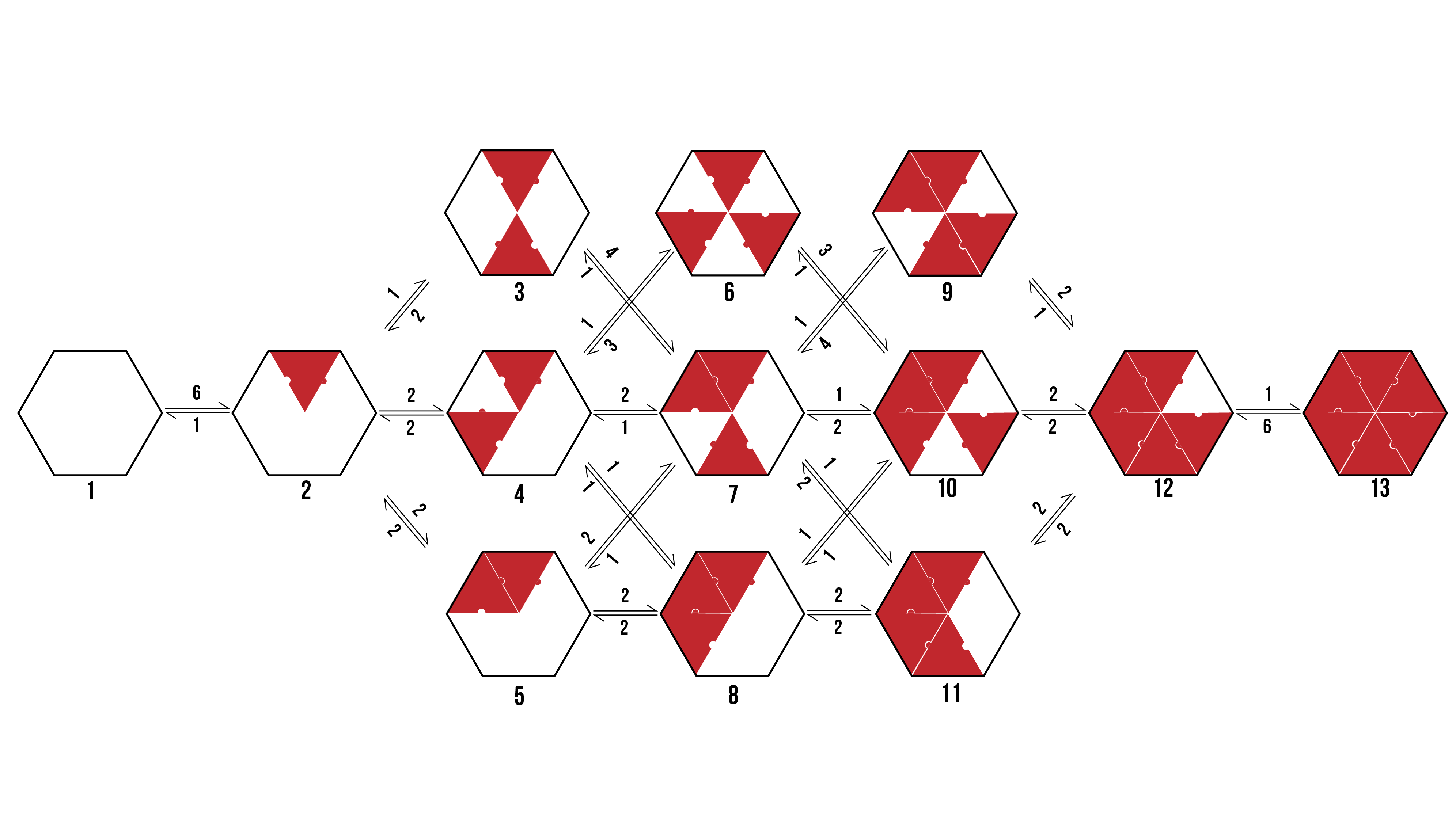
`\frac{d\[1]}{dt}=-6k_{0\rightarrow1}m\[1]+k_{1\rightarrow0}\[2]`
`\frac{d\[2]}{dt}=-k_{1\rightarrow0}\[2]+6k_{0\rightarrow1}m\[1]-k_{0\rightarrow1}m\[2]+2k_{1\rightarrow0}\[3]-2k_{0\rightarrow1}m\[2]+2k_{1\rightarrow0}\[4]-2k_{1\rightarrow2}m\[2]+2k_{2\rightarrow1}[5]`
`\frac{d\[3]}{dt}=-2k_{1\rightarrow0}\[3]+k_{0\rightarrow1}m\[2]-4k_{1\rightarrow2}m\[3]+k_{2\rightarrow1}[7]`
`\frac{d\[4]}{dt}=-2k_{1\rightarrow0}\[4]+2k_{0\rightarrow1}m\[2]-k_{0\rightarrow1}m\[4]+3k_{1\rightarrow0}\[6]-2k_{1\rightarrow2}m\[4]+k_{2\rightarrow1}\[7]-k_{2\rightarrow3}m\[4]+k_{3\rightarrow2}[8]`
`\frac{d\[5]}{dt}=-2k_{2\rightarrow1}\[5]+2k_{1\rightarrow2}m\[2]-2k_{0\rightarrow1}m\[5]+k_{1\rightarrow0}\[7]-2k_{1\rightarrow2}m\[5]+2k_{2\rightarrow1}[8]`
`\frac{d\[6]}{dt}=-3k_{1\rightarrow0}\[6]+k_{0\rightarrow1}m\[4]-3k_{2\rightarrow3}m\[6]+k_{3\rightarrow2}[10]`
`\frac{d\[7]}{dt}=-k_{2\rightarrow1}\[7]+3k_{1\rightarrow2}m\[3]-k_{2\rightarrow1}\[7]+2k_{1\rightarrow2}m\[4]-k_{1\rightarrow0}\[7]+2k_{0\rightarrow1}m\[5]-k_{2\rightarrow3}m\[7]`
`+2k_{3\rightarrow2}\[11]-k_{1\rightarrow2}m\[7]+2k_{2\rightarrow1}\[10]-k_{1\rightarrow2}m\[7]+4k_{2\rightarrow1}[9]`
`\frac{d\[8]}{dt}=-k_{3\rightarrow2}\[8]+k_{2\rightarrow3}m\[4]-2k_{2\rightarrow1}\[8]+2k_{1\rightarrow2}m\[5]-2k_{1\rightarrow2}m\[8]+2k_{2\rightarrow1}\[11]-k_{0\rightarrow1}m\[8]+k_{1\rightarrow0}[10]`
`\frac{d\[9]}{dt}=-4k_{2\rightarrow1}\[9]+k_{1\rightarrow2}m\[7]-2k_{2\rightarrow3}m\[9]+k_{3\rightarrow2}[12]`
`\frac{d\[10]}{dt}=-k_{3\rightarrow2}\[10]+3k_{2\rightarrow3}m\[6]-2k_{2\rightarrow1}\[10]+k_{1\rightarrow2}m\[7]-k_{1\rightarrow0}\[10]+k_{0\rightarrow1}m\[8]-2k_{2\rightarrow3}m\[10]+2k_{3\rightarrow2}[12]`
`\frac{d\[11]}{dt}=-2k_{3\rightarrow2}\[11]+k_{2\rightarrow3}m\[7]-2k_{2\rightarrow1}\[11]+2k_{1\rightarrow2}m\[8]-2k_{1\rightarrow2}m\[11]+2k_{2\rightarrow1}[12]`
`\frac{d\[12]}{dt}=-k_{3\rightarrow2}\[12]+2k_{2\rightarrow3}m\[9]-2k_{3\rightarrow2}\[12]+2k_{2\rightarrow3}m\[10]-2k_{2\rightarrow1}\[12]+2k_{1\rightarrow2}m\[11]-k_{2\rightarrow3}m\[12]+6k_{3\rightarrow2}[13]`
`\frac{d\[13]}{dt}=-6k_{3\rightarrow2}\[13]+k_{2\rightarrow3}m[12]`
Figure 13: We can change inputted rate constants to fit experimental data.
Whilst time constraints precluded us from extensively measuring the various neighbour-cases experimentally, and thus determining the above binding constants, future work could allow extraction of these constants. By inputting them into the above equation, we can theoretically predict the self-assembly of hexamers!
The below plot was extracted by inputting rate constants of `k_(1→0)/k_(0→1) =10^(-5) M`, `k_(2→1)/k_(1→2) =10^(-5) M` and `k_(3→2)/k_(2→3) =10^(-5) M`. The concentration of protein was taken as `20mM`, and the initial concentration of empty templates as `20μM`. This information corresponds with binding events that do not depend on neighbouring protein subunits. This would be consistent with a very small interaction strength between neighbouring subunits.
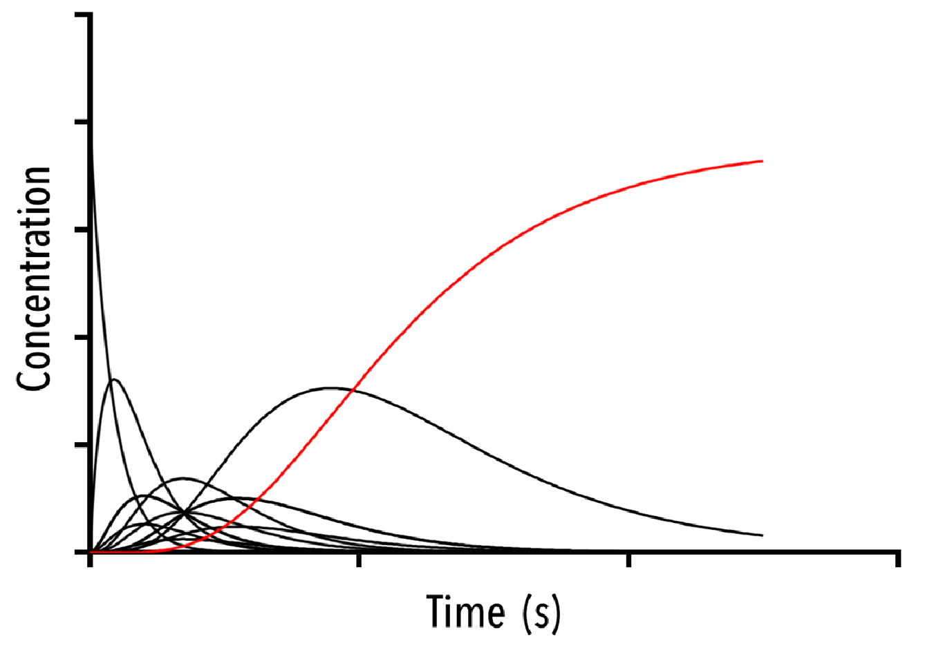
Figure 12: An example output of the Hexamer simulation. The red line is the overall hexamer formation, whilst the black lines represent the transitional states. By inputting rate constants for the zero, one and two-neighbour case, we can view changes in the output plot at thus predict the behaviour of capsid self-assembly
The red curve indicates the increase of full hexamer templates over time. As we can see, the concentration of full templates approaches the initial concentration of empty templates (described from the line that is initially non-zero). As such, we note that the equilibrium position of this function is such that the templates fill up completely. This best facilitates hexamerisation. Additionally, we can observe the prominent intermediate states.
Conclusion
We have successfully built, from the ground up, a model accounting for the self-assembly of capsid proteins. This model allows us, firstly, to develop experiments which test the zero, one and two neighbour cases outlined above, and extract the binding constants associated with each of these states. From this information alone, we can construct a theoretical binding curve for pentamer and hexamer formation, which may be compared with experimentally measured data.
Of particular merit is the ease of use, and flexibility of application, involved in this model. By simply changing a number of inputs, including effective and solution concentration, and approximations of kinetic constants, we can output curves which can be compared with SPR and BLItz data. Thus, prior to any in-depth analysis of our experimental results, we can assess the likely cause of particular experimental outcomes. In particular, we notice the standard sigmoidal curve shape apparent in the majority of outputted graphs. However, there are cases where the equilibrium does not result in all templates become full, or causes the templates to shed proteins over long periods of time. As such, we can qualitatively compare graph forms with experimental data prior to any quantitative analysis. This will give a general idea of the mechanism of assembly of capsid proteins in solution.
In addition, by considering self-assembly of proteins as a pathway of binding events, we can created a structure within which to build a model for any similar system. By identifying discrete bound states, and observing the interaction between these states, a set of differential equations may be set up and solved.
As the output of this model is not just the overall binding curve observed on SPR, but also the intermediate states required to get to a final hexamer/pentamer structure, we can easily visualise the likely pathways of formation. This gives us insight into the in vivo formation of pentamer and hexamer structures, and may suggest particular environments within which self-assembly is best facilitated.
This model could further be developed by adding layers of complexity previously not considered. For example, the wild-type capsid protein readily dimerizes in solution. Whilst we have shown, using SAXS, that the crystal monomer structure is almost identical to the solution monomer structure, it would appear that the dimer is a much more complicated beast. It is possible that, to form a hexamer or other self-assembled aggregate, the dimer must undergo a conformational change before binding with it’s neighbour. As such, an additional ‘unfurling’ term would need to be incorporated into the model, and could explain why pentamer and hexamer structures are rarely observed in solution at low concentrations.
References
- Adamson CS. & Jones IM. The molecular basis of HIV Capsid assembly – five years of progress. Rev Med Viron 14(2), 107-21 (2004).
- Heymann J. et al. Irregular and semi-regular polyhedral models for Rous sarcoma virus cores. Comput Math Methods Med 9(3-4).
- Pronillos O. et al. X-Ray Structures of the Hexameric Building Block of the HIV Capsid Cell 137(7), 1282-92 (2009).
- Huang Z et al. Tris-Nitrilotriacetic Acids of Subnanomolar Affinity Towards Hexahistidine Tagged Molecules Bioconjugate Chem 20(8), 1667-72 (2009)
- Li L. et al. Structural Analysis and Optimization of the Covalent Association between SpyCatcher and a Peptide Tag J Mol Biol 426(2) 309-17 (2014).
- Cohen S. et al. From Macroscopic Measurements to Microscopic Mechanisms of Protein Aggregation J Mol Biol 421(2-3), 160-71 (2012)
- Knowles TP et al. An Analytical Solution to the Kinetics of Breakable Filament Assembly Science 326(5959) 1533-7 (2009)
- Mesil G. et al. Molecular Mechanisms of Protein Aggregation from Global Fitting of Kinetic Models Nature Protocols 11, 252-72 (2016).
- Erdi, P. & Toth, J. Mathematical Models of Chemical Reactions: Theory and Applications of Deterministic and Stochasic Models Manchester University Press (1989)
- Ginnell R. & Simha R. On the Kinetics of Polymerization Reactions J Am Chem Soc 65(4), 715-27 (1943)